Analyzing all of the data in a worksheet can help you make better decisions. Creating a PivotTable from sheet data is a great way to summarize, analyze, explore, and present your data by freely moving and filtering data fields.

PivotCharts help you visualize this data. While a PivotChart shows data series, categories, and chart axes the same way as a standard chart, it also gives you the same interactive and dynamic controls you get from a PivotTable.

Convert Your Data into a Table

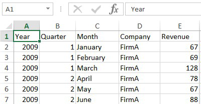
1. Click the top left-most cell in your data array.

• Most likely cell A1

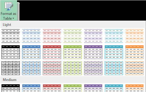
2. In the Styles group under the Home tab, click the Format as Table button and select any style.

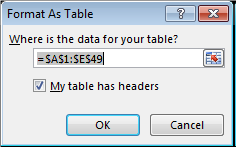
3. In the Format As Table dialogue, confirm the area of your table and check the My table has headers box.

• Confirm that the marching border includes your whole data array.

4. Click OK.

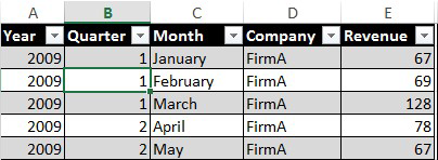
5. Your new table will appear in the style that you selected at Step 2.

Convert Your Table into a PivotTable

1. Click any cell inside of the new table.

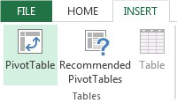
2. Click the Pivot Table button in the Tables group under the Insert tab.

3. In the Create PivotTable dialogue, click the New Worksheet radio to place the PivotTable on a separate worksheet.

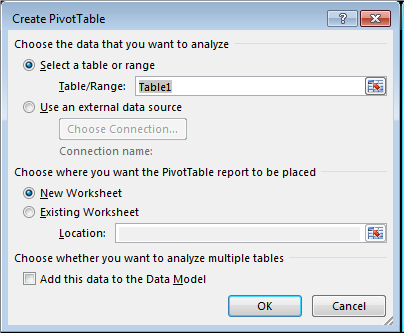
4. Click OK

Pivot Your Data

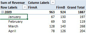
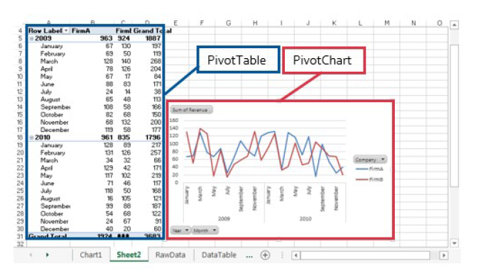
1. The PivotTable Report appears on the left side of the new worksheet.

• The PivotTable will be empty until Fields are selected from the Fields Pane on the right.
• A Field is created from each of the column headers in your original table.

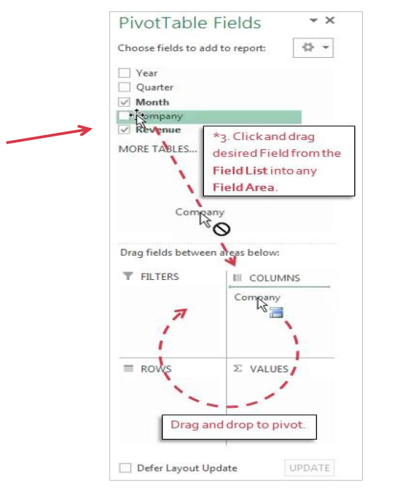
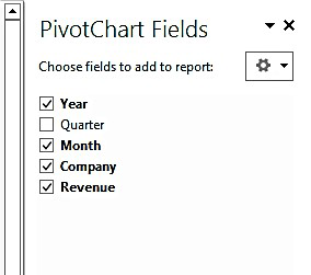
2. In the Fields Pane on the right, you will find the Field List at the top and the Field Area divided into four areas below.

3. Click and drag desired fields into any quadrant of the Field Area.*

• Drag Fields freely from quadrant to quadrant to change the layout of the PivotTable (on the left).
• This is what it means to “pivot.”

4. Pivot your Fields in the Fields Areas until your PivotTable meets your needs and is easy to analyze.

5. Remove a Field from the Report by unchecking its box in the Field List above.

 

Insert a PivotChart

1. Click any cell in the PivotTable.

2. Click the Insert tab in the ribbon.

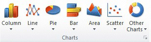
3. In the Charts group, select the chart style you’d like.

4. The new PivotChart will insert on the same sheet as the PivotTable.

• To avoid crowding, move the PivotChart to a new sheet.

5. Click the PivotChart.

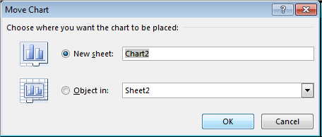
6. In the Design tab of the PivotChart Tools, click the Move Button in the Location group.

7. In the Move Chart dialogue, click the New Sheet radio.

• Optionally, change the name of the new sheet.

8. Click OK

 

Filter the PivotChart Fields

The PivotChart will be found on a new sheet apart from any other tables in the workbook. Like the PivotTable, the PivotChart can be updated by pivoting fields in the Pivot Pane on the right side of the sheet.

1. PivotChart tools are found in contextual ribbon tabs. These tabs are only visible with the chart is actively selected.

2. Like tables, charts are dynamic and can be changed by pivoting Fields in the Field Pane.

• Fields in tables and charts can be filtered to show only the data you want to see in the Report.

3. Hover over the Field on which you’d like to apply the filter.
Example: Field = Company

4. Click the dropdown arrow that appears to the right of the Field.

5. Apply any of three types of filter:

• Selection – Use check boxes to hide items.
• Rule – Set criteria either to Label (field name) or Value
  (data)
• Search – Type a word, or phrase to display only items that match the typed text.
• A funnel icon will will display next to the Field with the Filter.

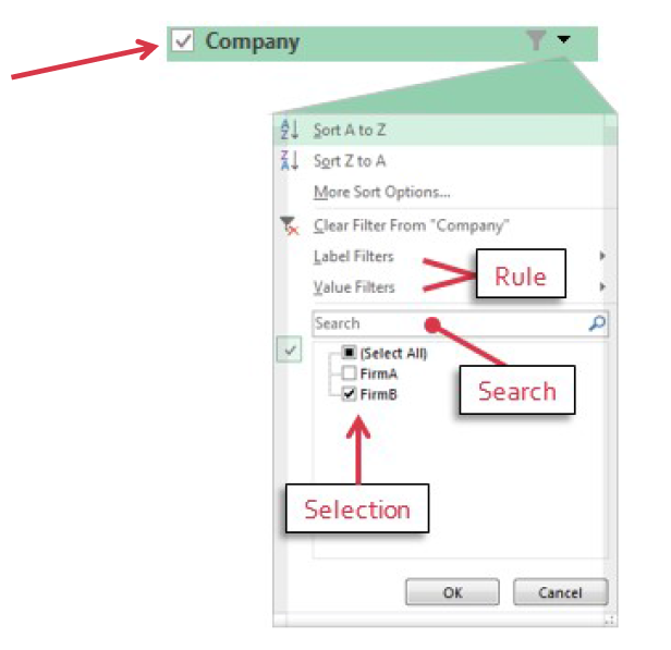
6. Click Clear Filter From “Field” to remove the filter.

 

If you have any questions or comments regarding the steps outlined in this document, please contact UHD TLS Training Services by calling (713) 221-8200, or by sending an email to ttlctraining@uhd.edu.